Visualization-Oriented Progressive Time Series Transformation
Xin Chen1
Lingyu Zhang2
Huaiwei Bao2
Wei Lu1
Eugene Wu3
Xiaohui Yu4
Yunhai Wang1
1Renmin University of China
2Shandong University
3Columbia University
4York University
Accepted by ACM SIGMOD 2026
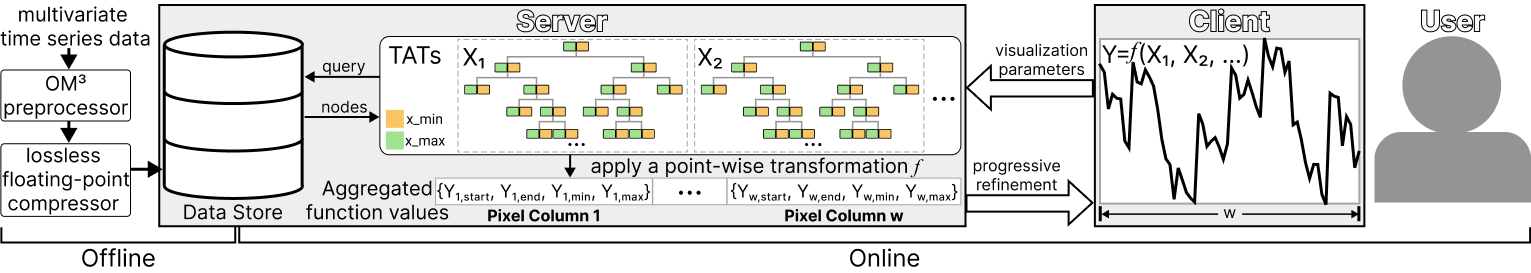
Figure 1:
Overview of our system PIVOT for exploring compressed large-scale time series stored in memory on a remote server.
Abstract:
Visual analysis of large time-series data often requires transformations over multivariate time series. Existing methods struggle to meet interactive response time requirements, relying on full transformations that incur high computation costs. We propose a visualization-oriented transformation system PIVOT that incrementally generates accurate visualizations by selectively transforming only essential data samples. At its core is a transformation-aware query mechanism that efficiently computes point-wise transformations by leveraging cached hierarchical data on the server. To support responsive interaction, we introduce a pixel-based error-bound guarantee that estimates the accuracy of intermediate visualizations without requiring a reference, enabling a balance between latency and visual fidelity. Experiments show that PIVOT achieves highly accurate visualizationswith interactive responsetimes, outperforming existing error-free methods by up to an order of magnitude on billion-scale datasets.
Source Code: github.com/ChenXin360104/PIVOT
Results:
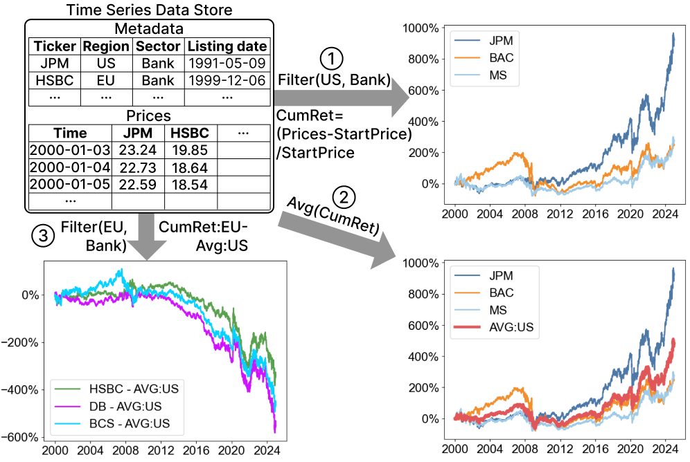
Figure 2: Visual analysis of multiple time series from a dataset of NYSE-listed stocks. Analysts may casually apply and compose various point-wise transformations to explore interesting patterns, expecting timely and highly accurate visualizations.
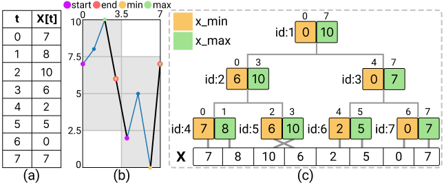
Figure 3: Illustration of M4 and our proposed TAT representation with a sample time series in (a). (b) The corresponding line charts with two pixel columns: the blue line connects all data points, while the black line uses only M4-aggregated samples in each pixel column. (c) The corresponding TAT structure, where each node stores the minimum and maximum values and the associated time interval.
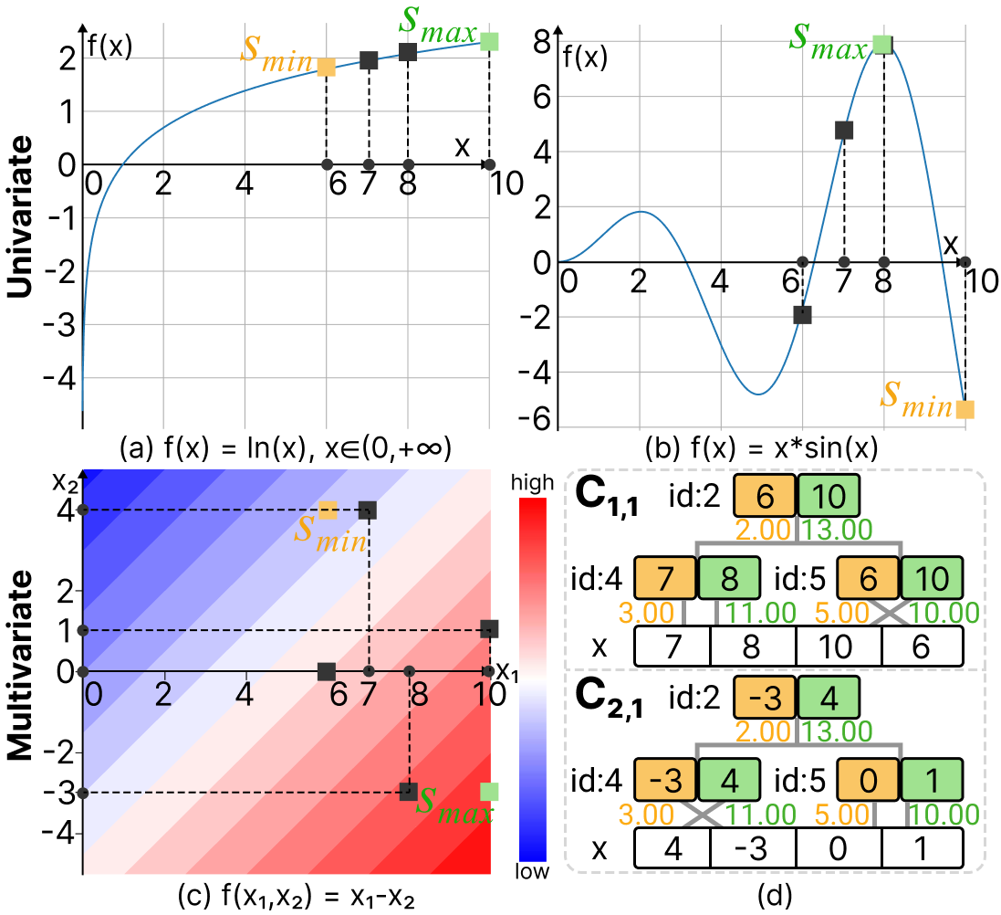
Figure 4: Illustration of how our solution handles three types of transformation functions: (a) monotonic univariate, (b) non-monotonic univariate, and (c) bivariate. In all cases, the input time series has values {7, 8, 10, 6}, represented by black dots within a single pixel column. The corresponding function values are shown as black squares, while yellow and green squares mark the minimum and maximum function values within the domain, respectively. In (c), an additional time series {4, -3, 0, 1} is used, and the corresponding TAT structures are illustrated in (d).
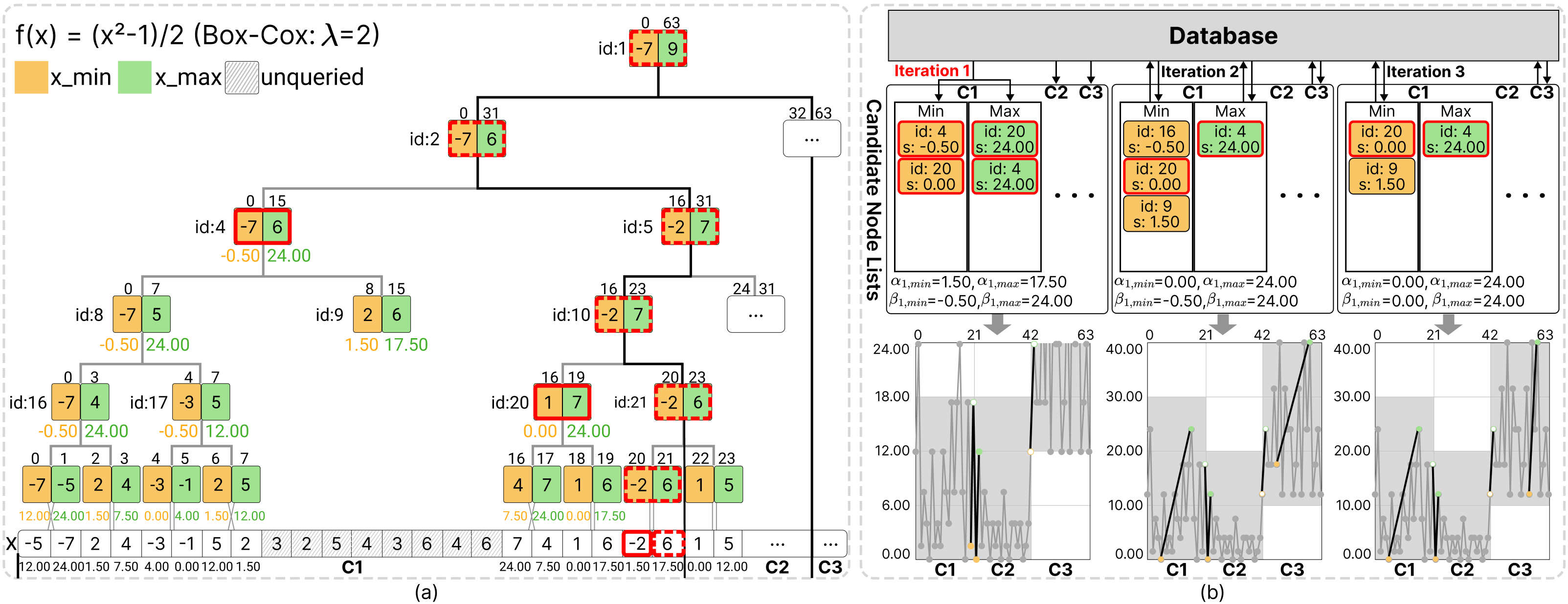
Figure 5: Illustration of the query mechanism Q on a time series of length 64 over a canvas with three pixel columns. (a) For the non-monotonic function f(x) = (x2 - 1) / 2, Q retrieves aggregated values from the TAT, with node scores shown below. (b) Evolution of candidate lists α and 𝛽 over the query process, alongside corresponding progressive visualizations. The ground truth f(X), shown in gray, is for reference only; it is not computed during execution.
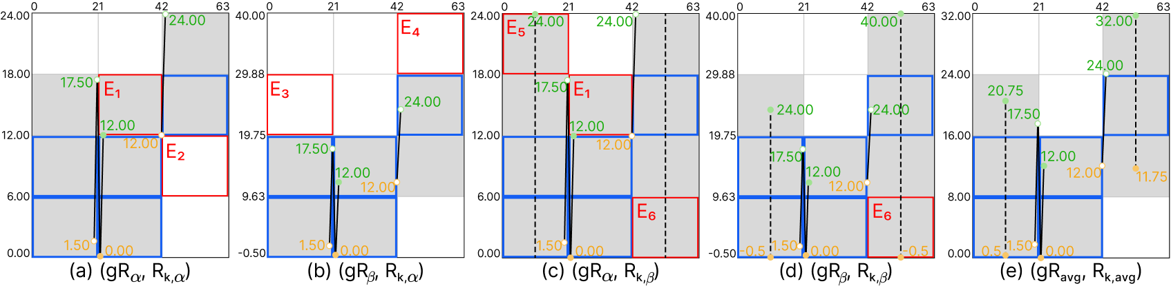
Figure 6: Illustration of pixel errors under different combinations of Rk and gR. (a-d) The four extreme rasterization cases and (e) our average estimation approach using α and 𝛽 values obtained in the first iteration. Red and blue boxes indicate erroneous pixels relative to the final visualization in Figure 5 (b) and consistently rasterized pixels across all four cases, respectively. Black dashed lines serve as virtual guides for rasterization between Rk that do not correspond to valid results.
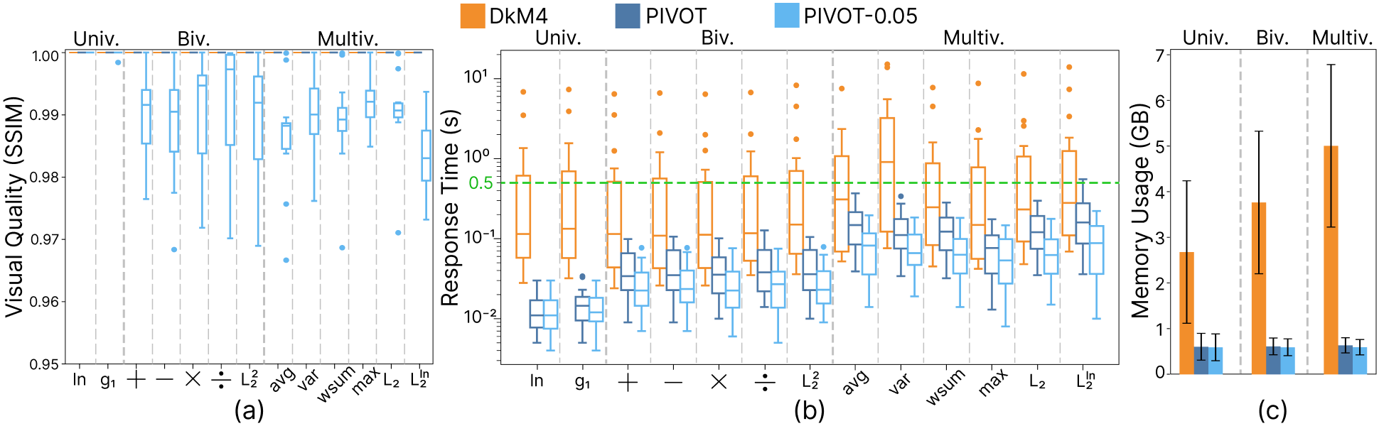
Figure 7: Performance comparison of three systems using 13 representative transformation functions covering univariate, bivariate, and multivariate cases evaluated on all datasets: (a) SSIM, (b) response time, and (c) memory usage.
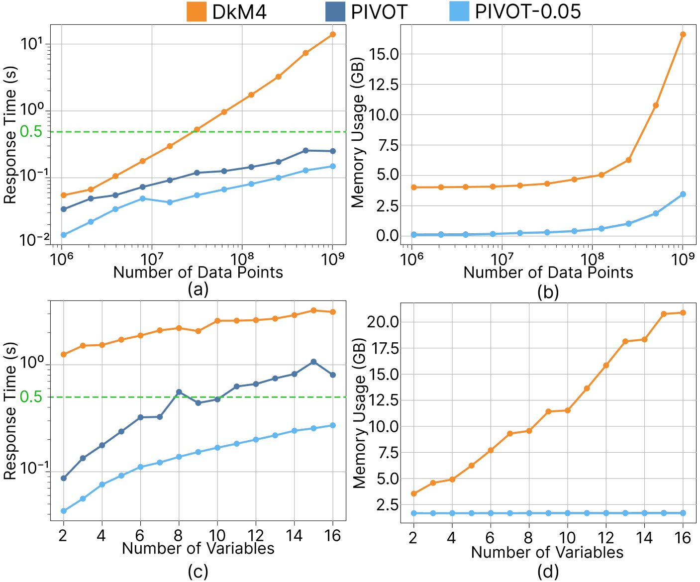
Figure 8: Response time (a,c) and memory usage (b,d) of the three systems under varying (a,b) numbers of data points and (c,d) numbers of input variables when applying the transformation L2ln(X) to the synthesized time-series datasets.
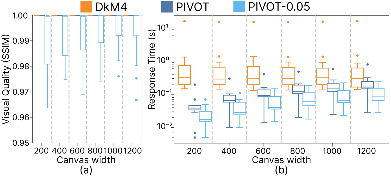
Figure 9: Results of evaluation metrics on the largest real-world dataset Power as the canvas width varies: (a) SSIM scores and (b) response time.
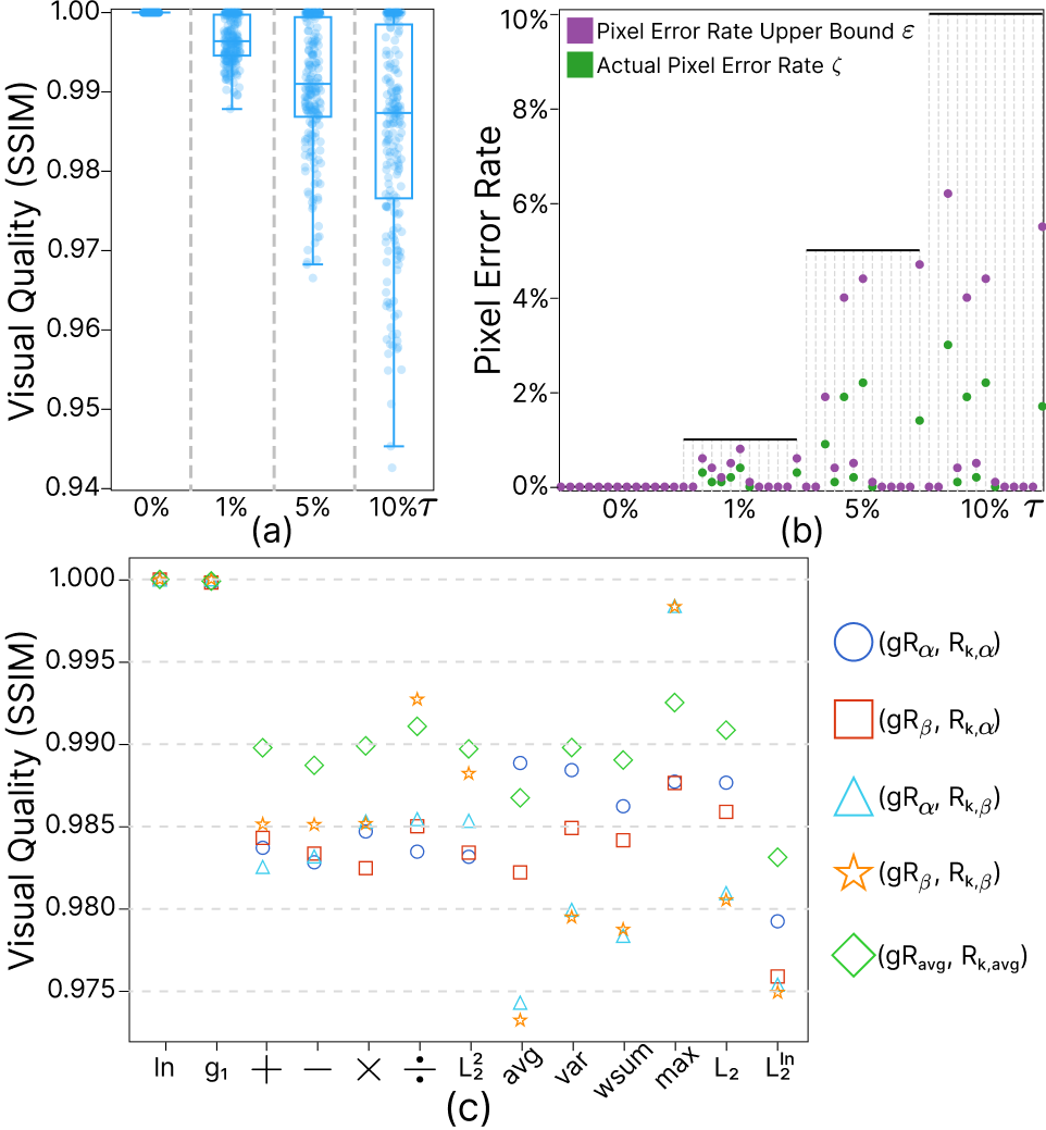
Figure 10: Performance under varying pixelerror rate thresh- olds 𝜏. (a) The boxplots summarize the SSIM scores across all datasets. (b) The dot plot shows the relationship between pixel error rate upper bound ε and the actual pixel rate 𝜁 on the Power dataset. (c) The dot plot displays the mean SSIM scores for various configurations with a fixed 𝜏 = 5%.
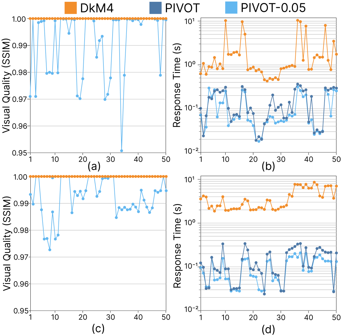
Figure 11: Interactive performance on the real-world dataset Taxi (a, b) and synthetic dataset Syn5B (c, d): (a, c) SSIM scores; (b, d) response times.
Materials:
 |
 |
| Paper (3.27M) | Supp. (2.94M) |
Acknowledgements:
This work is supported by the grants of the National Key R&D Program of China under Grant 2022ZD0160805, NSFC (No.62132017 and No.U2436209), the Shandong Provincial Natural Science Foundation (No.ZQ2022JQ32), the Beijing Natural Science Foundation (L247027), the Fundamental Research Funds for the Central Universities, the Research Funds of Renmin University of China, and Big Data and Responsible Artificial Intelligence for National Governance, Renmin University of China.